TidyTuesday dataset of December 2, 2025

import pandas as pd
import matplotlib.pyplot as plt
import seaborn as sns
import textwrap

sechselaeuten = pd.read_csv('https://raw.githubusercontent.com/rfordatascience/tidytuesday/main/data/2025/2025-12-02/sechselaeuten.csv')
sechselaeuten

	year	duration	tre200m0	tre200mn	tre200mx	sre000m0	sremaxmv	rre150m0	record
0	1923	60.00	16.67	7.03	32.47	247.43	56.33	73.97	False
1	1952	6.00	18.73	9.10	33.70	269.70	61.67	93.67	False
2	1953	8.00	16.67	7.17	29.97	209.53	48.67	157.90	False
3	1956	4.00	15.07	6.80	28.77	172.83	39.67	174.90	False
4	1958	8.00	17.00	8.23	30.67	230.30	53.00	177.87	False
...	...	...	...	...	...	...	...	...	...
62	2021	12.95	17.97	9.83	30.13	190.13	44.67	169.37	False
63	2022	37.98	20.40	11.40	34.40	284.66	66.67	82.17	True
64	2023	57.00	20.07	10.57	33.23	253.37	59.33	110.70	True
65	2024	NaN	19.50	10.33	31.40	214.59	50.67	98.93	True
66	2025	26.50	19.60	10.50	32.80	250.81	58.67	126.80	True

67 rows × 9 columns

sechselaeuten.dropna(inplace=True)
sechselaeuten.columns

Index(['year', 'duration', 'tre200m0', 'tre200mn', 'tre200mx', 'sre000m0',
       'sremaxmv', 'rre150m0', 'record'],
      dtype='object')

duration_max = sechselaeuten.loc[sechselaeuten['duration'].idxmax()]
duration_min = sechselaeuten.loc[sechselaeuten['duration'].idxmin()]
duration_max['year'], duration_min['year'], duration_max['duration'], duration_min['duration']

(np.int64(1923), np.int64(1956), np.float64(60.0), np.float64(4.0))

sechselaeuten[sechselaeuten['record']==True]

	year	duration	tre200m0	tre200mn	tre200mx	sre000m0	sremaxmv	rre150m0	record
25	1983	24.33	19.07	9.10	31.37	207.14	48.67	52.83	True
36	1994	21.92	19.13	9.57	31.70	217.18	51.33	85.03	True
45	2003	5.70	21.67	11.30	34.57	281.84	67.00	83.50	True
56	2015	20.65	20.17	9.63	33.17	259.30	61.00	80.60	True
58	2017	9.93	19.53	10.13	32.37	226.42	53.33	119.87	True
59	2018	20.52	20.17	9.40	32.63	267.33	62.67	80.33	True
60	2019	17.73	19.73	9.83	33.50	251.68	59.00	109.37	True
63	2022	37.98	20.40	11.40	34.40	284.66	66.67	82.17	True
64	2023	57.00	20.07	10.57	33.23	253.37	59.33	110.70	True
66	2025	26.50	19.60	10.50	32.80	250.81	58.67	126.80	True

bg_color = "#550000"
text_color = "#ED8E8E"
plot_color1 = '#BA55D3'
sns.set_theme(style="white", rc={
    "font.family": "monospace", 
    "text.color": text_color,   
    "axes.labelcolor": text_color, 
    "xtick.color": text_color,     
    "ytick.color": text_color      
})
custom_palette = {
    True: "#FC0000",
    False: plot_color1
}
fig, ax = plt.subplots(figsize=(8,5))
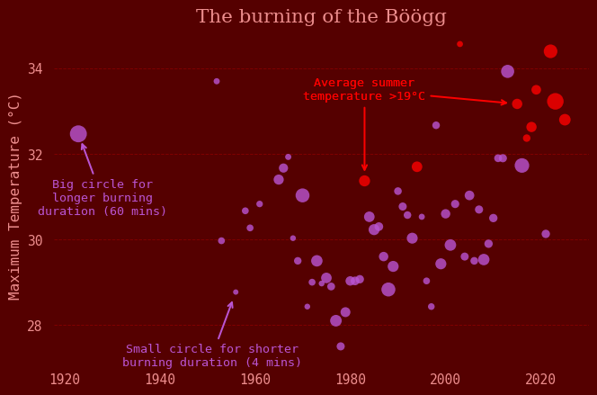
sns.scatterplot(data=sechselaeuten, x='year', y='tre200mx', hue='record', size='duration',\
                sizes=(20, 200), alpha=0.8, edgecolor='none', palette=custom_palette, legend=False)
sns.despine(bottom=True, left=True)
fig.patch.set_facecolor(bg_color)
ax.set_facecolor(bg_color)
plt.xlabel("")
plt.ylabel("Maximum Temperature (°C)")
plt.grid(True, axis='y', which='major', color='#820000', linestyle='--', linewidth=0.7)
plt.yticks(range(28, 35, 2))
#title = "Timeline of yearly maximum temperature. Years with average temp > 19°C are red."
#plt.title(textwrap.fill(title, width=50))
plt.title('The burning of the Böögg', fontsize=16, family='Serif')
ax.annotate(
    textwrap.fill(f"Big circle for longer burning duration ({duration_max['duration']:.0f} mins)", 20),   # the text
    xy=(duration_max['year'], duration_max['tre200mx']),           # point to annotate
    xytext=(duration_max['year']+5, duration_max['tre200mx'] - 1.5),   # position of text
    ha="center", va="center", fontsize=10, color=plot_color1,
    arrowprops=dict(
        arrowstyle="->", color=plot_color1, lw=1.5, shrinkB=7.5
    )
)
ax.annotate(
    textwrap.fill(f"Small circle for shorter burning duration ({duration_min['duration']:.0f} mins)", 25),
    xy=(duration_min['year'], duration_min['tre200mx']),           # point to annotate
    xytext=(duration_min['year']-5, duration_min['tre200mx'] - 1.5),   # position of text
    ha="center", va="center", fontsize=10, color=plot_color1,
    arrowprops=dict(
        arrowstyle="->", color=plot_color1, lw=1.5, shrinkB=7.5
    )
)
ax.annotate(
    textwrap.fill("Average summer temperature >19°C", 25),
    xy=(1983, sechselaeuten[sechselaeuten['year']==1983]['tre200mx']),   
    xytext=(1983, 33.5),  
    ha="center", va="center", fontsize=10, color="#FC0000",
    arrowprops=dict(
        arrowstyle="->", color="#FC0000", lw=1.5, shrinkB=7.5
    )
)
ax.annotate(
    textwrap.fill("Average summer temperature >19°C", 25),
    xy=(2015, sechselaeuten[sechselaeuten['year']==2015]['tre200mx']),   
    xytext=(1983, 33.5),  
    ha="center", va="center", fontsize=10, color="#FC0000",
    arrowprops=dict(
        arrowstyle="->", color="#FC0000", lw=1.5, shrinkB=7.5
    )
)
plt.savefig("sechselaeuten.png", dpi=300, bbox_inches='tight')
plt.show()