TidyTuesday dataset of November 4, 2025

import pandas as pd
import matplotlib.pyplot as plt
from matplotlib.ticker import FuncFormatter
import seaborn as sns
from scipy.stats import skew, kurtosis
import textwrap

flint_mdeq = pd.read_csv('https://raw.githubusercontent.com/rfordatascience/tidytuesday/main/data/2025/2025-11-04/flint_mdeq.csv')
flint_vt = pd.read_csv('https://raw.githubusercontent.com/rfordatascience/tidytuesday/main/data/2025/2025-11-04/flint_vt.csv')

flint_mdeq

	sample	lead	lead2	notes
0	1	0	0.0	NaN
1	2	104	NaN	sample removed: house had a filter
2	3	10	10.0	NaN
3	4	6	6.0	NaN
4	5	5	5.0	NaN
...	...	...	...	...
66	67	2	2.0	NaN
67	68	0	0.0	NaN
68	69	3	3.0	NaN
69	70	5	5.0	NaN
70	71	2	2.0	NaN

71 rows × 4 columns

sns.scatterplot(data=flint_mdeq, x='sample', y='lead')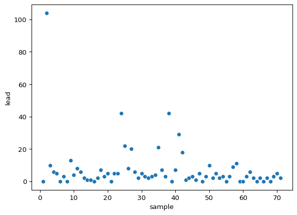

plt.scatter(flint_mdeq['sample'],flint_mdeq['lead2'])
#plt.scatter(flint_vt['sample'],flint_vt['lead'])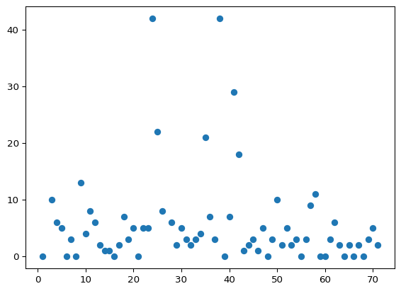

flint_mdeq.describe()

	sample	lead	lead2
count	71.000000	71.000000	69.000000
mean	36.000000	7.309859	5.724638
std	20.639767	14.347316	8.336461
min	1.000000	0.000000	0.000000
25%	18.500000	2.000000	2.000000
50%	36.000000	3.000000	3.000000
75%	53.500000	6.500000	6.000000
max	71.000000	104.000000	42.000000

desc = flint_mdeq[['lead','lead2']].describe().T[['mean','50%', 'min','max']]
desc

	mean	50%	min	max
lead	7.309859	3.0	0.0	104.0
lead2	5.724638	3.0	0.0	42.0

desc.plot(kind='bar', figsize=(10,6))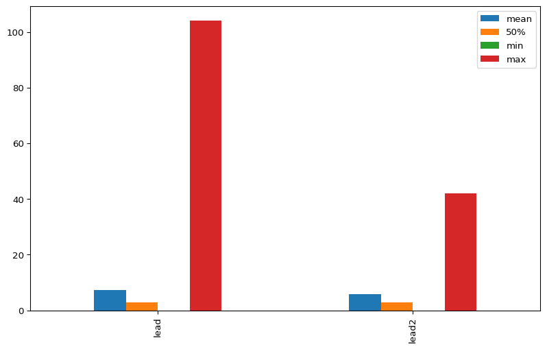

sns.swarmplot(flint_mdeq[['lead','lead2']])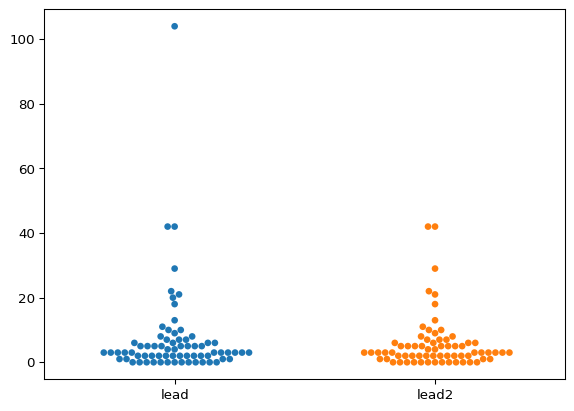

flint_mdeq

	sample	lead	lead2	notes
0	1	0	0.0	NaN
1	2	104	NaN	sample removed: house had a filter
2	3	10	10.0	NaN
3	4	6	6.0	NaN
4	5	5	5.0	NaN
...	...	...	...	...
66	67	2	2.0	NaN
67	68	0	0.0	NaN
68	69	3	3.0	NaN
69	70	5	5.0	NaN
70	71	2	2.0	NaN

71 rows × 4 columns

flint_mdeq['diff'] = flint_mdeq.apply(
    lambda row: row['lead'] if pd.isna(row['lead2']) else None,
    axis=1
)

d = flint_mdeq['lead2'].dropna()
print("Skewness:", skew(d))
print("Kurtosis:", kurtosis(d))

Skewness: 2.9376969574953016
Kurtosis: 9.133276189367894

melted = flint_mdeq[['lead', 'lead2','diff']].melt(var_name='Source', value_name='Lead Level')
fig,ax=plt.subplots(figsize=(6, 6))
ax2 = ax.twinx()
sns.swarmplot(x='Source', y='Lead Level', data=melted[melted['Source'].isin(['lead', 'lead2'])], size=6, hue='Source')
temp = melted[melted['Source']=='diff']
temp['Source'] = temp['Source'].str.replace('diff','lead')
plt.scatter(temp['Source'], temp['Lead Level'],marker='*', color='red',s=100,zorder=10, alpha=0.5)
desc.plot(ax=ax, alpha=0, legend=False)
ax.set_yticks(desc.loc['lead'])
ax2.set_yticks(desc.loc['lead2'])
#ax.grid(True, axis='y', color='#1f77b4')
yticks = ax.get_yticks()

# Get x-axis limits
xlim = ax.get_xlim()
x_half = (xlim[0] + xlim[1]) / 2  # midpoint of x-axis

# Draw custom horizontal lines from left to midpoint
for ytick in yticks:
    ax.hlines(y=ytick, xmin=xlim[0], xmax=x_half-0.1, color='#1f77b4', linestyle='--', linewidth=0.5)

#ax2.grid(True, axis='y', color='#ff7f0e')
yticks = ax2.get_yticks()

# Get x-axis limits
xlim = ax2.get_xlim()
x_half = (xlim[0] + xlim[1]) / 2  # midpoint of x-axis

# Draw custom horizontal lines from left to midpoint
for ytick in yticks:
    ax2.hlines(y=ytick, xmin=xlim[1], xmax=x_half+0.1, color='#ff7f0e', linestyle='--', linewidth=0.5)

ax.tick_params(axis='both', which='both', length=0)
ax2.tick_params(axis='both', which='both', length=0)
formatter = FuncFormatter(lambda val, pos: f'{val:.1f}')
ax2.yaxis.set_major_formatter(formatter)
ax.text(0.5, -1, 'Min',ha='center')
ax.text(0.5, 2.5, 'Median',ha='center')
ax.text(0.35, 7.5, 'Mean',ha='center', color='#1f77b4')
ax.text(0.6, 6, 'Mean',ha='center', color='#ff7f0e')
ax.text(0.35, 104, 'Max',ha='center', color='#1f77b4')
ax.text(0.6, 42, 'Max',ha='center', color='#ff7f0e')

ax.text(0,80,f'Skewness: {round(skew(flint_mdeq["lead"]),2)}', ha='center', color='#1f77b4')
ax.text(0,75,f'Kurtosis: {round(kurtosis(flint_mdeq["lead"]),2)}', ha='center', color='#1f77b4')

ax.text(1,80,f'Skewness: {round(skew(flint_mdeq["lead2"].dropna()),2)}', ha='center', color='#ff7f0e')
ax.text(1,75,f'Kurtosis: {round(kurtosis(flint_mdeq["lead2"].dropna()),2)}', ha='center', color='#ff7f0e')

plt.ylabel('')
sns.despine(left=True,bottom=True)
title="Distribution of Lead concentration in Flint water samples. The two leptokurtic distributions differ by two data points (red asterisks)."
plt.title('\n'.join(textwrap.wrap(title,50)), fontfamily='Serif', fontsize=14)
ax.set_facecolor('#EEEEEE')  
fig.set_facecolor('#EEEEEE')
plt.tight_layout()
plt.savefig('Flint_water.png', dpi=300, bbox_inches='tight')
plt.show()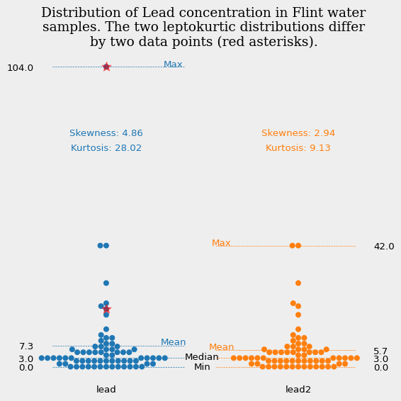

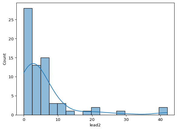
sns.histplot(flint_mdeq['lead2'], kde=True)
plt.show()