TidyTuesday dataset of October 21, 2025

import marimo as mo
import pandas as pd
import matplotlib.pyplot as plt
import seaborn as sns
import matplotlib.cm as cm
import matplotlib.colors as mcolors
import textwrap

historic_station_met = pd.read_csv('https://raw.githubusercontent.com/rfordatascience/tidytuesday/main/data/2025/2025-10-21/historic_station_met.csv')
station_meta = pd.read_csv('https://raw.githubusercontent.com/rfordatascience/tidytuesday/main/data/2025/2025-10-21/station_meta.csv')

historic_station_met

	station	year	month	tmax	tmin	af	rain	sun
0	aberporth	1941	1	NaN	NaN	NaN	74.7	NaN
1	aberporth	1941	2	NaN	NaN	NaN	69.1	NaN
2	aberporth	1941	3	NaN	NaN	NaN	76.2	NaN
3	aberporth	1941	4	NaN	NaN	NaN	33.7	NaN
4	aberporth	1941	5	NaN	NaN	NaN	51.3	NaN
...	...	...	...	...	...	...	...	...
39143	yeovilton	2024	8	22.2	12.8	0.0	27.4	141.1
39144	yeovilton	2024	9	18.3	10.7	0.0	142.8	107.6
39145	yeovilton	2024	10	16.2	8.1	0.0	102.0	85.2
39146	yeovilton	2024	11	11.7	5.1	7.0	88.6	48.8
39147	yeovilton	2024	12	10.5	5.0	1.0	29.6	27.9

39148 rows × 8 columns

historic_station_met['year'] = pd.to_datetime(historic_station_met['year']).astype(int)

bins = [1850, 1925, 1950, 1975, 2000, 2025]
labels = ['till 1925', '1926–1950', '1951–1975', '1976–2000', '2001 onwards']
historic_station_met['quarter'] = pd.cut(historic_station_met['year'], bins=bins, labels=labels)

historic_station_met['tdiff'] = historic_station_met['tmax']-historic_station_met['tmin']
historic_station_met['station'] = historic_station_met['station'].str.capitalize()

historic_station_met.columns

Index(['station', 'year', 'month', 'tmax', 'tmin', 'af', 'rain', 'sun',
       'quarter', 'tdiff'],
      dtype='object')

df_grp = historic_station_met.groupby(['station','year', 'month', 'quarter']).agg({
    'tmax': 'max',
    'tmin': 'min',
    'tdiff': 'mean',
    'af': 'sum',
    'rain': 'sum',
     'sun': 'sum'
}).reset_index()
df_grp

	station	year	month	quarter	tmax	tmin	tdiff	af	rain	sun
0	Aberporth	1853	1	till 1925	NaN	NaN	NaN	0.0	0.0	0.0
1	Aberporth	1853	1	1926–1950	NaN	NaN	NaN	0.0	0.0	0.0
2	Aberporth	1853	1	1951–1975	NaN	NaN	NaN	0.0	0.0	0.0
3	Aberporth	1853	1	1976–2000	NaN	NaN	NaN	0.0	0.0	0.0
4	Aberporth	1853	1	2001 onwards	NaN	NaN	NaN	0.0	0.0	0.0
...	...	...	...	...	...	...	...	...	...	...
381835	Yeovilton	2024	12	till 1925	NaN	NaN	NaN	0.0	0.0	0.0
381836	Yeovilton	2024	12	1926–1950	NaN	NaN	NaN	0.0	0.0	0.0
381837	Yeovilton	2024	12	1951–1975	NaN	NaN	NaN	0.0	0.0	0.0
381838	Yeovilton	2024	12	1976–2000	NaN	NaN	NaN	0.0	0.0	0.0
381839	Yeovilton	2024	12	2001 onwards	10.5	5.0	5.5	1.0	29.6	27.9

381840 rows × 10 columns

# Group by both station and year
grouped = historic_station_met.groupby(['station', 'year'])

# Dictionary to store correlation results
correlations = {}

# Loop through each (station, year) group
for (station, year), df_grp1 in grouped:
    # Compute correlation between 'rain' and 'sun'
    corr_matrix = df_grp1[['rain', 'sun']].corr()
    corr_value = corr_matrix.loc['rain', 'sun']

    # Store result with a tuple key
    correlations[(station, year)] = corr_value

correlation_df = pd.DataFrame.from_dict(
    correlations, orient='index', columns=['rain_sun_corr']
)

# Split the tuple index into two columns
correlation_df.index = pd.MultiIndex.from_tuples(correlation_df.index, names=['station', 'year'])
correlation_df = correlation_df.reset_index()

print(correlation_df)

        station  year  rain_sun_corr
0     Aberporth  1941            NaN
1     Aberporth  1942      -0.432952
2     Aberporth  1943      -0.527707
3     Aberporth  1944      -0.440227
4     Aberporth  1945      -0.251566
...         ...   ...            ...
3268  Yeovilton  2020      -0.653444
3269  Yeovilton  2021      -0.141005
3270  Yeovilton  2022      -0.438216
3271  Yeovilton  2023      -0.555453
3272  Yeovilton  2024      -0.234487

[3273 rows x 3 columns]

sns.scatterplot(data=correlation_df, x='year', y='rain_sun_corr', hue='station', alpha=0.5, legend=False)
plt.show()

df_grp[df_grp['quarter'] == '1926–1950']

	station	year	month	quarter	tmax	tmin	tdiff	af	rain	sun
1	Aberporth	1853	1	1926–1950	NaN	NaN	NaN	0.0	0.0	0.0
6	Aberporth	1853	2	1926–1950	NaN	NaN	NaN	0.0	0.0	0.0
11	Aberporth	1853	3	1926–1950	NaN	NaN	NaN	0.0	0.0	0.0
16	Aberporth	1853	4	1926–1950	NaN	NaN	NaN	0.0	0.0	0.0
21	Aberporth	1853	5	1926–1950	NaN	NaN	NaN	0.0	0.0	0.0
...	...	...	...	...	...	...	...	...	...	...
381816	Yeovilton	2024	8	1926–1950	NaN	NaN	NaN	0.0	0.0	0.0
381821	Yeovilton	2024	9	1926–1950	NaN	NaN	NaN	0.0	0.0	0.0
381826	Yeovilton	2024	10	1926–1950	NaN	NaN	NaN	0.0	0.0	0.0
381831	Yeovilton	2024	11	1926–1950	NaN	NaN	NaN	0.0	0.0	0.0
381836	Yeovilton	2024	12	1926–1950	NaN	NaN	NaN	0.0	0.0	0.0

76368 rows × 10 columns

##Plotting

col_palette = 'autumn_r' #'Wistia'
month_labels = ['J', 'F', 'M', 'A', 'M', 'J', 'J', 'A', 'S', 'O', 'N', 'D']
sns.set_context("talk", font_scale=2.2)  
bg_color = '#390099'
fg_color = '#eef4ed'

# Create a faceted stripplot

g = sns.catplot(
    data=df_grp,
    x='month',
    y='tmax',
    hue='tdiff',
    col='station',
    kind='strip',
    palette=col_palette,
    dodge=False,
    sharey=True,
    height=5,
    aspect=1.2,
    col_wrap=8,
    legend=False,
)
g.fig.patch.set_facecolor(bg_color)  

# Set axes background color
for ax in g.axes.flat:
    ax.set_facecolor(bg_color)  
    ax.tick_params(axis='y', colors=fg_color)
    for spine in ax.spines.values():
        spine.set_color(fg_color)

col_wrap = 8

for i, ax in enumerate(g.axes.flat):
    if i % col_wrap != 0:  # Not the first column in each row
        ax.set_ylabel('')
        ax.tick_params(axis='y', left=False, labelleft=False, colors=fg_color)
        ax.tick_params(axis='x', colors=fg_color)
        sns.despine(ax=ax,left=True)
    else:
        ax.tick_params(axis='x', colors=fg_color)

# Adjust layout
g.set_titles("{col_name}", color=fg_color)
g.set_axis_labels("", "")
g.set_xticklabels(month_labels, fontdict={'family': 'monospace', 'color': fg_color})
g.fig.text(-0.005, 0.5, 'Maximum temperature (°C)', va='center', rotation='vertical', color=fg_color)

norm = mcolors.Normalize(vmin=df_grp['tdiff'].min(), vmax=df_grp['tdiff'].max())
sm = cm.ScalarMappable(cmap='autumn_r', norm=norm)
sm.set_array([])  # Required for colorbar

#g.fig.subplots_adjust(right=0.85)
# Add the colorbar to the figure
cbar_ax = g.fig.add_axes([0.7, 0.08, 0.2, 0.01])  # [left, bottom, width, height]
cbar = g.fig.colorbar(sm, cax=cbar_ax, orientation='horizontal')
cbar.set_label('Temperature Difference', color=fg_color)

# Change tick label color
cbar.ax.xaxis.set_tick_params(color=fg_color)  # Tick marks
for label in cbar.ax.get_xticklabels():
    label.set_color(fg_color)  # Tick label text
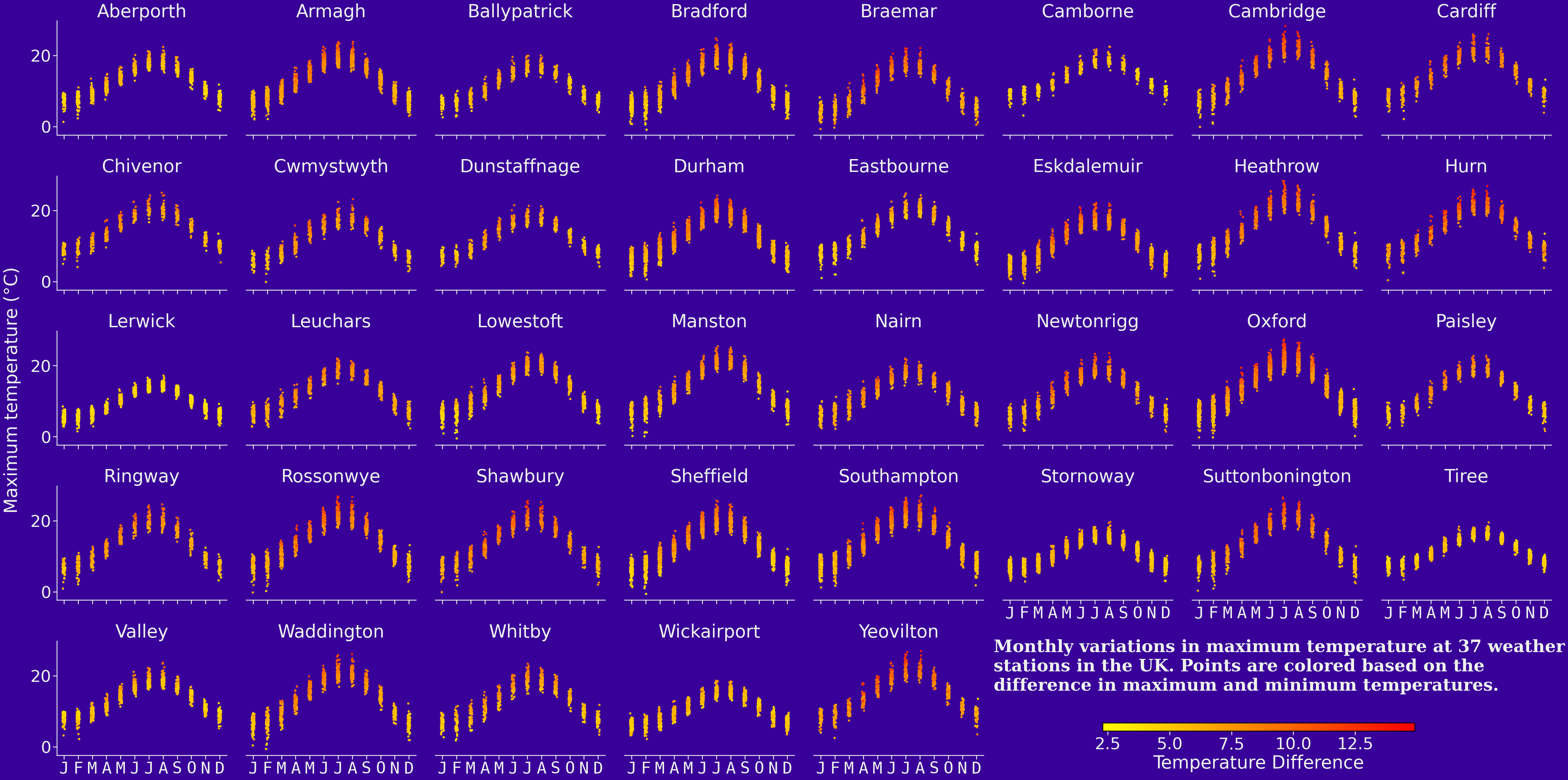
title = 'Monthly variations in maximum temperature at 37 weather stations in the UK. Points are colored based on the difference in maximum and minimum temperatures.'    

g.fig.text(0.63, 0.13,textwrap.fill(title, width=55), color=fg_color, family='Serif', fontweight='bold', fontsize=38)           
plt.tight_layout()
plt.savefig("UK_weather.png", dpi=300, bbox_inches='tight', pad_inches=0.2)
plt.show()